COMPLEX NETWORK MEASURES

  RATE EQUATIONS FOR TRANSCRIPTION

  COMPLEX NETWORK MEASURES

• Simple graph or network: a group of N nodes (vertices) among which there exist L undirected connections (links, edges), identical in strength.

• Directed graph: a group of nodes among which connections are directed.

• Weighted network: a group of nodes among which connections are not identical in strength, but carry a weight.

• Bipartite network: a network with more than one type of node, in which connections only exist between different node types (the definition can be relaxed to a network were most, but not all links run between vertices of different types).

• Adjacency matrix A: an N × N matrix representing the network, whose elements are equal to 1 when there is a link from node i to j, zero otherwise.

• Degree distribution: probability that a node of a network, chosen uniformly at random, has degree k.

• Scale-free network: a network in which the tail of the degree distribution follows a power law (strictly speaking, the term scale-free implies P(k) decays as k to a power - γ, however, it is often used for networks where the tail of the distribution follows a power-law).

• Degree exponent γ: the power law exponent of the (tail of the) degree distribution.

• Scale-free model: a growing network model proposed by Barabási and Albert. The model builds a simple graph starting from a small connected group of nodes, to which new nodes are added one by one. These new nodes connect to m old nodes with probabilites that increase linearly with the degree of the old nodes.

• Shortest path (geodesic path): the smallest collection of links that form a path through the network from one vertex to another.

• Diameter D: the length of the largest geodesic path in a network.

• Small-world network: a network in which the average shortest path length grows logarithmically (or slower) with N.

• Node betweennes (betweenness centrality or load): the number of shortest paths between nodes of the network that run through a given node.

• Edge betweennes: the number of shortest paths between nodes of the network that run through a given edge.

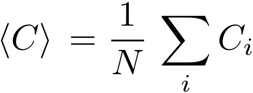
• Clustering coefficient C: the fraction of connections that are realized between the neighbours of a node:

  

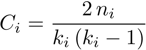
  where n_i denotes the number of links connecting the k_i neighbors of node i. (The average clustering coefficient is given by

  

• Assortativity coefficient: a measure of the tendency of links to run among nodes that are similar in some respect. If the similarity is described by a scalar quantity (most often the node’s degree), then the assortativity coefficient is given by

  

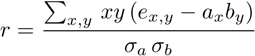
  where x (y) is the scalar at the origin (end) of a link, e_(x,y) denotes the fraction of all edges in the network that go from nodes with value x to ones with value y, a_x (b_y) is the fraction of edges that start (end) at a link vith values x (y), and σ_a (σ_b ) is the standard deviations of the distributions of a_x (b_y) values.

• Modularity Q: the number of links between nodes within the same community minus the number expected by chance:

  

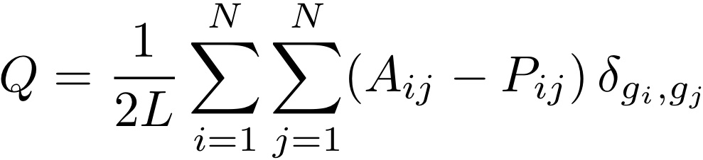
  where node i (j) belongs to the community g_i (g_j). P_(ij) gives the expected number of links between two nodes if the network is random with respect to communities. In the simplest case, in which the null model is a random network, P_(ij) = 2 L/N. A more suitable assumption is P_(ij) = (k_i x k_j)/2L, which preserves the degree distribution of the network in question.

  RATE EQUATIONS FOR TRANSCRIPTION

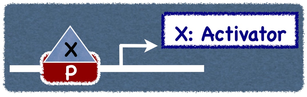
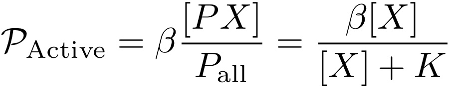
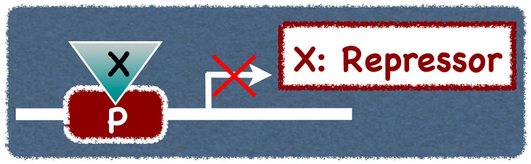
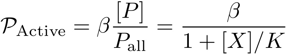
• Rate of transcription P: number of mRNA molecules transcribed in unit time (Β denotes the rate of transcription from a promoter that is 100% occupied, or saturated, while K is the ratio of complex dissociation and formation rates):
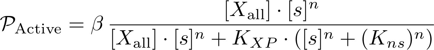
  • Promoter driven by one activator:

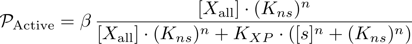
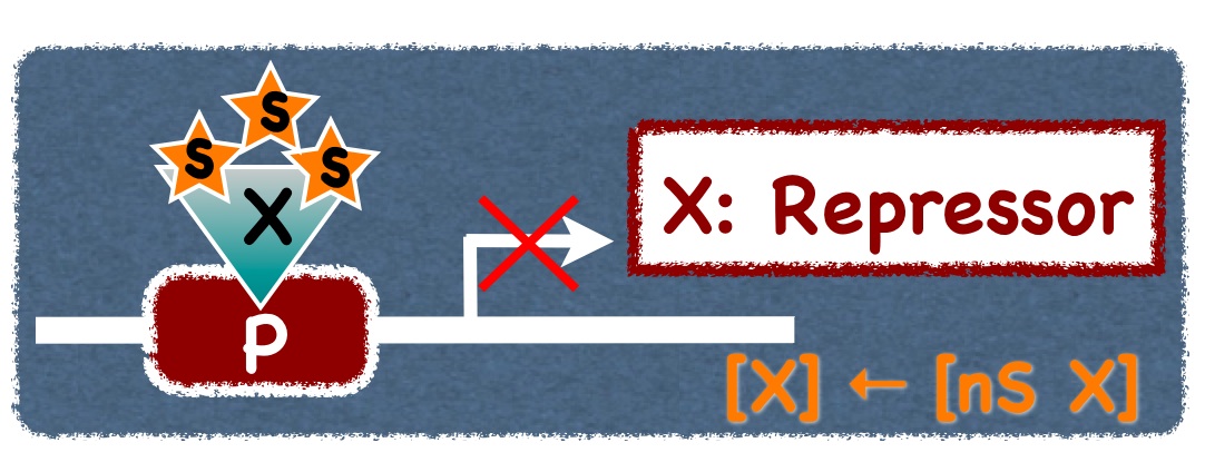
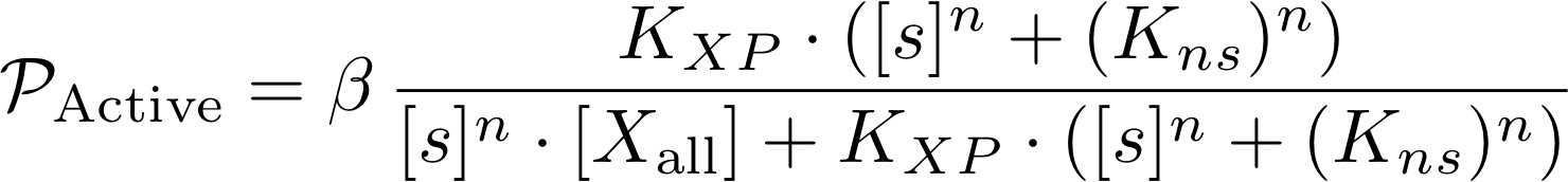
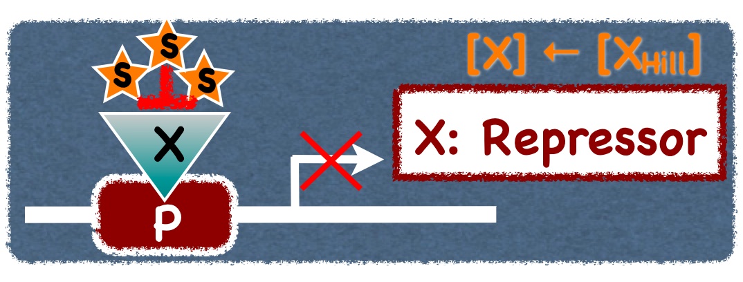
  • Active promoter scilenced by one repressor:

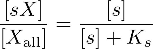
  • Inducer - transcription factor complex formation (fraction of transcription factors in complex):
    • Michaelis-Menten equation for non-cooperative inducer binding:

      		Fraction of TF's in complex		Fraction of free TF's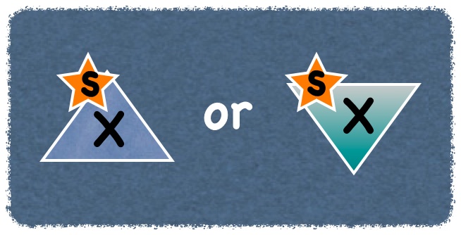

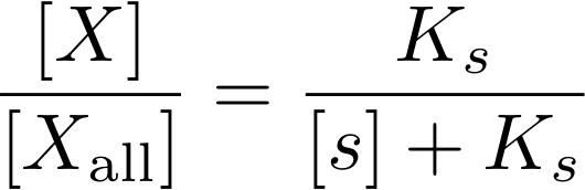
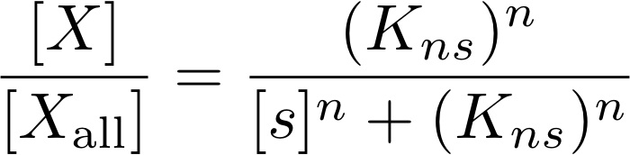
    • Hill's equation for cooperative inducer binding (complexes require n inducers):

      		Fraction of TF's in complex		Fraction of free TF's

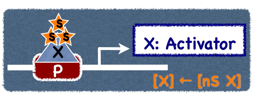
  • Promoter driven by a inducer-responsive activator (Michaelis-Menten menten inducer binding ← n = 1):
    • Inducer activates the transcription factor:

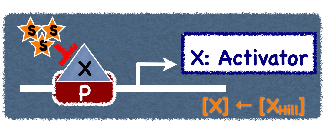
    • Inducer represses the transcription factor:

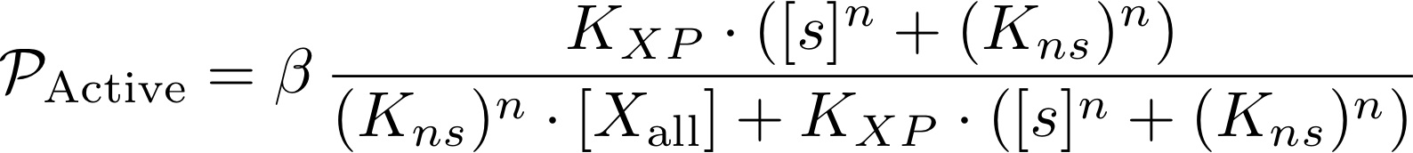
  • Promoter driven by a inducer-responsive repressor (Michaelis-Menten menten inducer binding ← n = 1):
    • Inducer activates the transcription factor:

    • Inducer represses the transcription factor: